Pre -Requisites
- Linux Machine (I’m using Ubuntu 18.04)
- Python 3 + PIP3 ( + Know what environments are and how to use it)
- VSCode
Create a file named setup-1.sh and paste the code below:
# Python3
sudo apt-get install python3 -y;
py3_version=$(python3 --version);
echo -e "\e[31m$py3_version\e[39m";

# Pip3
sudo apt-get install python3-pip -y;
pip3_version=$(pip3 --version);
echo -e "\e[31m$pip3_version\e[39m";

# VSCode
sudo snap install vscode --classic;
Be sure that setup-1.sh has 775 permissions (sudo chmod 775 setup-1.sh).
Execute in your terminal ./setup-1.sh in order to install required software (tested in Ubuntu 18.04).
Computer Vision (Review Links)
Before you put hands on the following example, is better you review the following Videos (better if you follow the order):
- C4W1L01 Computer Vision
- C4W1L02 Edge Detection Examples
- C4W1L03 More Edge Detection
- C4W1L04 Padding
- Which Activation Function Should I Use?
Python Virtual Environment:
- Create a directory for your new project (called vision-example).
- Inside that directory, create a file called setup-2.sh, and give it execute permissions (
sudo chmod 775 setup-2.sh). - Also, inside that dir, create a file called requirements.txt
- Execute in your terminal:
./setup-2.sh
Inside requirements.txt you must paste:
tensorflow==2.0.0-alpha0
numpy==1.16
Inside setup-2.sh you must paste:
pip3 install virtualenv;
virtualenv PythonEnvironment --python=python3;
source PythonEnvironment/bin/activate;
pip3 install -r requirements.txt && \
deactivate;
Library to use
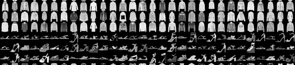
zalandoresearch / fashion-mnist
Fashion-MNIST is a dataset consisting of a training set of 60,000 examples and a test set of 10,000 examples. Each example is a 28×28 grayscale image, associated with a label from 10 classes.
Labels
Each training and test example is assigned to one of the following labels:
| Label | Description |
|---|---|
| 0 | T-shirt/top |
| 1 | Trouser |
| 2 | Pullover |
| 3 | Dress |
| 4 | Coat |
| 5 | Sandal |
| 6 | Shirt |
| 7 | Sneaker |
| 8 | Bag |
| 9 | Ankle boot |
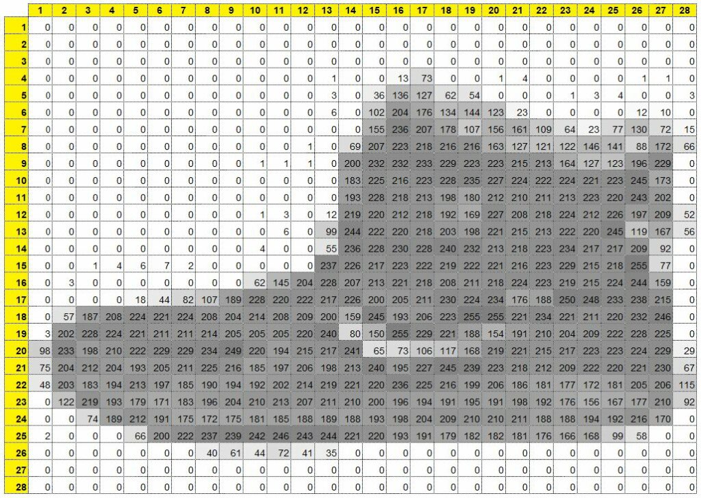
The 60,000 training elements of the library are images of 28×28 pixels. Each pixel stores a number from 0 to 255 (represents a scale from white to gray)
If you take the first element of the set and put it in excell, we can use conditional format in order to understand better how the information is stored.
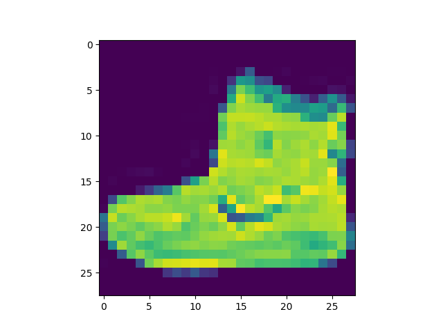
The label of the “element[0]” is 9 (Ankle boot).
The “element[0]” (first element of the set of 60,000 elements) is a matrix of 28×28.
print(training_labels[0])
print(training_images[0])
Problem to solve
We need to clasify (“predict”) 10,000 images using one of the 10 labels available (T-shirt/top, Trouser, Pullover, Dress, Coat, Sandal, Shirt, Sneaker, Bag, Ankle boot) per each “prediction”.
In order to achieve that, we will perform the following actions:
- Import images to use (training images & test images). Library incorporated in Tensorflow.
- Normalize data. Neural networks works better using values from 0 to 1, so we will “normalize” the available data (divide each value per the max value). Since each value goes from 0 to 255, the max value is 255.
- Create a model (specify quantity of layers, activation function, loss function, optimizer, number of epochs).
- Train the model with 60,000 examples and calculate the loss (the error in %) and the accuracy in %. Since each one of the 60,000 images is labeled (from 0 to 10), the NN (Neural Network) can predict and verify the error of each prediction.
- Predict the label of the 10,000 images
Running the example
Let’s create a file called vision-nmist.py and paste the following code:
import tensorflow as tf
print(tf.__version__)

mnist = tf.keras.datasets.fashion_mnist
(training_images, training_labels), (test_images, test_labels) = mnist.load_data()

import matplotlib as matplt
print(matplt.__version__)

import matplotlib.pyplot as plt
plt.imshow(training_images[0])
print(training_labels[0])
print(training_images[0])

training_images  = training_images / 255.0
test_images = test_images / 255.0

model = tf.keras.models.Sequential([tf.keras.layers.Flatten(),
                                    tf.keras.layers.Dense(128, activation=tf.nn.relu),
                                    tf.keras.layers.Dense(10, activation=tf.nn.softmax)])
model.compile(optimizer = 'adam', #tf.train.AdamOptimizer(),
              loss = 'sparse_categorical_crossentropy',
              metrics=['accuracy'])

model.fit(training_images, training_labels, epochs=5)

model.evaluate(test_images, test_labels)

classifications = model.predict(test_images)

print(classifications[0])
print(classifications[9999])

print(test_labels[0])
print(test_labels[9999])

plt.show()
To run the code:
PythonEnvironment/bin/python3 vision-nmist.py
NOTES:
Sequential: That defines a SEQUENCE of layers in the neural network
Flatten: just takes the square (matrix of 28×28) and turns it into a 1 dimensional set (784×1).
Our NN has an input layer of 784 elements and an output layer of 10 elements. Also, we only have set 01 hidden layer of 128 neurons (in the image we have 02 hidden layers). Each one of the 784 elements is the value of a pixel (from 0 to 255).
Image taken from But what is a Neural Network? | Deep learning, chapter 1
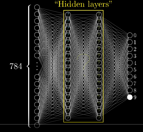
Dense: Adds a layer of neurons. The input layer needs to fit the shape of input data. The output layer needs to fit the shape of output data. For example, you need to put an output layer of 10 since there are 10 labels, and you need to put an input layer of 784 neurons, since the number of inputs of each image is 784 pixels (28×28). The hidden layers could have different values.
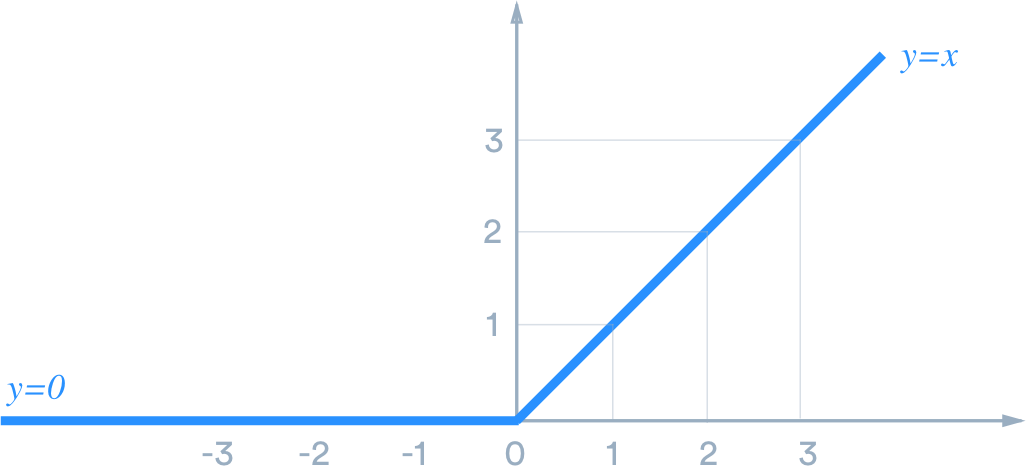
Relu: Each layer of neurons need an “activation function” to tell them what to do. There’s lots of options, but just use these for now. Relu effectively means “If X>0 return X, else return 0” — so what it does it it only passes values 0 or greater to the next layer in the network.
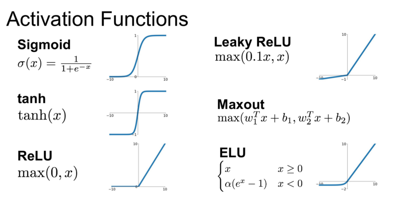
Softmax: takes a set of values, and effectively picks the biggest one, so, for example, if the output of the last layer looks like [0.1, 0.1, 0.05, 0.1, 9.5, 0.1, 0.05, 0.05, 0.05], it saves you from fishing through it looking for the biggest value, and turns it into [0,0,0,0,1,0,0,0,0] — The goal is to save a lot of coding!
To Normalize data:
training_images = training_images / 255.0
test_images = test_images / 255.0
To Create the Model:
model = tf.keras.models.Sequential([
tf.keras.layers.Flatten(),
tf.keras.layers.Dense(128, activation=tf.nn.relu),
tf.keras.layers.Dense(10, activation=tf.nn.softmax)])
To Train the Neural Network:
model.fit(training_images, training_labels, epochs=5)
To Evaluate the “loss” using 10,000 data never seen by the NN. This can be calculated, since those new images has its own label.
model.evaluate(test_images, test_labels)
To predict clasification of 10,000 images:
classifications = model.predict(test_images)
To show images 1 and 10,000 of the array of predicitions/clasifications :
print(classifications[0])
print(classifications[9999])
To show the real labels of images 1 and 10,000:
print(test_labels[0])
print(test_labels[9999])
Review Results:
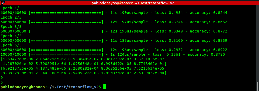
As you can see:
There were 05 iterations (60,000 images trained on each iteration). Last accuracy obtained is 0,8922 (89,22 %)
The evaluation of 10,000 images gives us an accuracy of 87,80 % (less than value obtained during training)
The first prediction (for image “0”= first image) gives us a vector (length = 10) with values from 0 to 1. The index with the higher value corresponds to the number of label. For this first vector, the max value is 8.7748462e-01. And this corresponds to index =9 (Label 9 = Ankle boot).
The second prediction (for image “9999” = last image) gives us a vector (length = 10) with values from 0 to 1. The max value is 9.8922950e-01 and corresponds to index = 5 (Label 5 = Sandal).
As you can see, NN works beter with numbers, so the results says “5” and “9”, and we need to go to the table in order to know “what this number means”. This is in order to avoid BIAS related to Language.